Exploring IA at the Edge!

Image Recognition, Object and Pose Detection using Tensorflow Lite on a Raspberry Pi

Introduction

What is Edge (or Fog) Computing?

Gartner defines edge computing as: “a part of a distributed computing topology in which information processing is located close to the edge — where things and people produce or consume that information.”

In other words, edge computing brings computation (and some data storage) closer to the devices where it’s data are being generated or consumed (especially in real-time), rather than relying on a cloud-based central system far away. With this approach, data does not suffer latency issues, reducing the amount of cost in transmission and processing. In a way, it is a kind of “return to the recent past,” where all the computational work was done locally on a desktop and not in the cloud.

Edge computing was developed due to the exponential growth of IoT devices connected to the internet for either receiving information from the cloud or delivering data back to the cloud. And many Internet of Things (IoT) devices generate enormous amounts of data during their operations. 

Edge computing provides new possibilities in IoT applications, particularly for those relying on machine learning (ML) for tasks such as object and pose detection, image (and face) recognition, language processing, and obstacle avoidance. Image data is an excellent addition to IoT, but also a significant resource consumer (as power, memory, and processing). Image processing “at the Edge”, running classics AI/ML models, is a great leap!

Tensorflow Lite – Machine Learning (ML) at the edge!!

Machine Learning can be divided into two separated process: Training and Inference, as explained in Gartner Blog:

• Training: Training refers to the process of creating a machine learning algorithm. Training involves using a deep-learning framework (e.g., TensorFlow) and training dataset (see the left-hand side of the above figure). IoT data provides a source of training data that data scientists and engineers can use to train machine learning models for various cases, from failure detection to consumer intelligence.
• Inference: Inference refers to the process of using a trained machine-learning algorithm to make a prediction. IoT data can be used as the input to a trained machine learning model, enabling predictions that can guide decision logic on the device, at the edge gateway, or elsewhere in the IoT system (see the right-hand side of the above figure).

TensorFlow Lite is an open-source deep learning framework that enables on-device machine learning inference with low latency and small binary size. It is designed to make it easy to perform machine learning on devices, “at the edge” of the network, instead of sending data back and forth from a server.

Performing machine learning on-device can help to improve:

• Latency: there’s no round-trip to a server
• Privacy: no data needs to leave the device
• Connectivity: an Internet connection isn’t required
• Power consumption: network connections are power-hungry

TensorFlow Lite (TFLite) consists of two main components:

• The TFLite converter, which converts TensorFlow models into an efficient form for use by the interpreter, and can introduce optimizations to improve binary size and performance.
• The TFLite interpreter runs with specially optimized models on many different hardware types, including mobile phones, embedded Linux devices, and microcontrollers.

In summary, a trained and saved TensorFlow model (like model.h5) can be converted using TFLite Converter in a TFLite FlatBuffer (like model.tflite) that will be used by TF Lite Interpreter inside the Edge device (as a Raspberry Pi), to perform inference on a new data.

For example, I trained from scratch a simple CNN Image Classification model in my Mac (the “Server” on the above figure). The final model had 225,610 parameters to be trained, using as input the CIFAR10 dataset: 60,000 images (shape: 32, 32, 3). The trained model (cifar10_model.h5) had a size of 2.7Mb. Using the TFLite Converter, the model used on Raspberry Pi (model_cifar10.tflite) became with 905Kb (around 1/3 of original size). Making inference with both models (.h5 at Mac and .tflite at RPi) leaves the same results. Both notebooks can be found at GitHub.

Raspberry Pi — TFLite Installation 

It is also possible to train models from scratch at Raspberry Pi, and for that, the full TensorFlow package is needed. But once what we will do is only the inference part, we will install just the TensorFlow Lite interpreter.

The interpreter-only package is a fraction the size of the full TensorFlow package and includes the bare minimum code required to run inferences with TensorFlow Lite. It includes only the tf.lite.InterpreterPython class, used to execute .tflite models.

Let’s open the terminal at Raspberry Pi and install the Python wheel needed for your specific system configuration. The options can be found on this link: Python Quickstart. For example, in my case, I am running Linux ARM32 (Raspbian Buster — Python 3.7), so the command line is:

$ sudo pip3 install https://dl.google.com/coral/python/tflite_runtime-2.1.0.post1-cp37-cp37m-linux_armv7l.whl

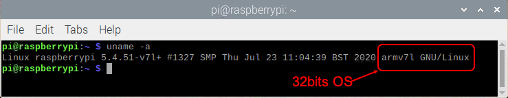
If you want to double-check what OS version you have in your Raspberry Pi, run the command:

$ uname -

As shown on image below, if you get …arm7l…, the operating system is a 32bits Linux.

Installing the Python wheel is the only requirement for having TFLite interpreter working in a Raspberry Pi. It is possible to double-check if the installation is OK, calling the TFLite interpreter at the terminal, as below. If no errors appear, we are good.

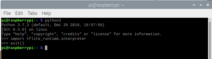
Image Classification

Introduction

One of the more classic tasks of IA applied to Computer Vision (CV) is Image Classification. Starting on 2012, IA and Deep Learning (DL) changed forever, when a convolutional neural network (CNN) called AlexNet (in honor of its leading developer, Alex Krizhevsky), achieved a top-5 error of 15.3% in the ImageNet 2012 Challenge. According to The Economist, “Suddenly people started to pay attention (in DL), not just within the AI community but across the technology industry as a whole

This project, almost eight years after Alex Krizhevsk, a more modern architecture (MobileNet), was also pre-trained over millions of images, using the same dataset ImageNet, resulting in 1,000 different classes. This pre-trained and quantized model was so, converted in a .tflite and used here. 

First, let’s on Raspberry Pi move to a working directory (for example, Image_Recognition). Next, it is essential to create two subdirectories, one for models and another for images:

$ mkdir images
$ mkdir models

Once inside the model’s directory, let’s download the pre-trained model (in this link, it is possible to download several different models). We will use a quantized Mobilenet V1 model, pre-trained with images of 224×224 pixels. The zip file that can be downloaded from TensorFlow Lite Image classification, using wget:

$ cd models
$ wget https://storage.googleapis.com/download.tensorflow.org/models/tflite/mobilenet_v1_1.0_224_quant_and_labels.zip

Next, unzip the file:

$ unzip mobilenet_v1_1.0_224_quant_and_labels

Two files are downloaded:

• mobilenet_v1_1.0_224_quant.tflite: TensorFlow-Lite transformed model
• labels_mobilenet_quant_v1_224.txt: The ImageNet dataset 1,000 Classes Labels

Now, get some images (for example, .png, .jpg) and save them on the created images subdirectory. 

On GitHub, it is possible to find the images used on this tutorial.

Raspberry Pi OpenCV and Jupyter Notebook installation

OpenCV (Open Source Computer Vision Library) is an open-source computer vision and machine learning software library. It is beneficial as a support when working with images. If very simple to install it on a Mac or PC is a little bit “trick” to do it on a Raspberry Pi, but I recommend to use it.

Please follow this great tutorial from Q-Engineering to install OpenCV on your Raspberry Pi: Install OpenCV 4.4.0 on Raspberry Pi 4. Although written for the Raspberry Pi 4, the guide can also be used without any change for the Raspberry 3 or 2.

Next, Install Jupyter Notebook. It will be our development platform.

$ sudo pip3 install jupyter
$ jupyter notebook

Also, during OpenCV installation, NumPy should have been installed, if not do it now, same with MatPlotLib.

$ sudo pip3 install numpy
$ sudo apt-get install python3-matplotlib

And it is done! We have everything in place to start our AI journey to the Edge!

Image Classification Inference

Create a fresh Jupyter Notebook and follow bellow steps, or download the complete notebook from GitHub.

Import Libraries:

import numpy as np
import matplotlib.pyplot as plt
import cv2
import tflite_runtime.interpreter as tflite

Load TFLite model and allocate tensors:

interpreter = tflite.Interpreter(model_path=’./models/mobilenet_v1_1.0_224_quant.tflite’)
interpreter.allocate_tensors()

Get input and output tensors:

input_details = interpreter.get_input_details()
output_details = interpreter.get_output_details()

input details will give you the info needed about how the model should be feed with an image:

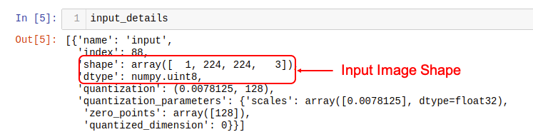
The shape of (1, 224x224x3), informs that an image with dimensions: (224x224x3) should be input one by one (Batch Dimension: 1). The dtype uint8, tells that the values are 8bits integers

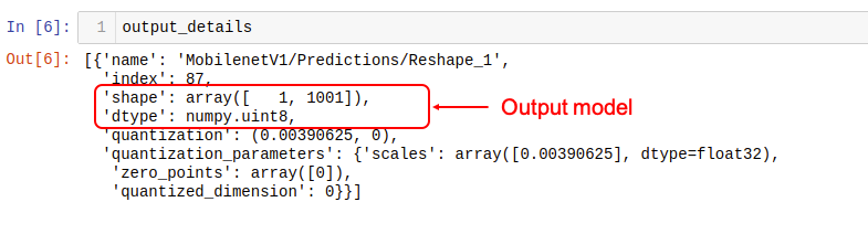
The output details show that the inference will result in an array of 1,001 integer values (8 bits). Those values are the result of the image classification, where each value is the probability of that specific label be related to the image.

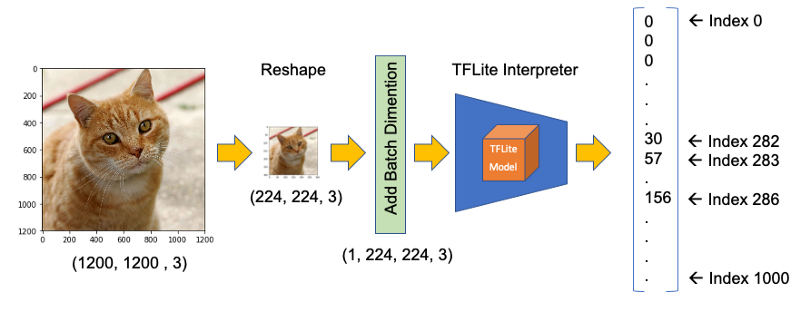
For example, suppose that we want to classify an image wich shape is (1220, 1200, 3). First, we will need to reshape it to (224, 224, 3) and add a batch dimension of 1, as defined on input details: (1, 224, 224, 3). The inference result will be an array with 1001 size, as shown below:

The steps to code those operations are:

1. Input image and convert it to RGB (OpenCV reads an image as BGR):

image_path = './images/cat_2.jpg'
image = cv2.imread(image_path)
img = cv2.cvtColor(image, cv2.COLOR_BGR2RGB)

2. Pre-process the image, reshaping and adding batch dimension:

img = cv2.resize(img, (224, 224))
input_data = np.expand_dims(img, axis=0)

3. Point the data to be used for testing and run the interpreter:

interpreter.set_tensor(input_details[0]['index'], input_data)
interpreter.invoke()

4. Obtain results and map them to the classes:

predictions = interpreter.get_tensor(output_details[0][‘index’])[0]

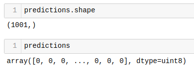
The output values (predictions) varies from 0 to 255 (max value of an 8bit integer). To obtain a prediction that will range from 0 to 1, the output value should be divided by 255. The array’s index, related to the highest value, is the most probable classification of such an image.

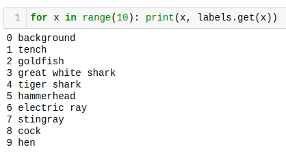
Having the index, we must find to what class it appoint (such as car, cat, or dog). The text file downloaded with the model has a label associated with each index that goes from 0 to 1,000.

Let’s first create a function to load the .txt file as a dictionary:

def load_labels(path):
    with open(path, 'r') as f:
        return {i: line.strip() for i, line in enumerate(f.readlines())}

And create a dictionary named labels and inspecting some of them:

labels = load_labels('./models/labels_mobilenet_quant_v1_224.txt')

Returning to our example, let’s get the top 3 results (highest probabilities):

top_k_indices = 3
top_k_indices = np.argsort(predictions)[::-1][:top_k_results]

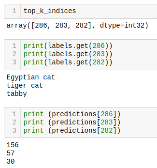
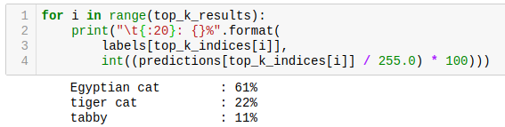
We can see that the 3 top indices are related to cats. The prediction content is the probability associated with each one of the labels. As explained before, dividing by 255., we can get a value from 0 to 1. Let’s create a loop to go over the top results, printing label and probabilities:

for i in range(top_k_results):
    print("\t{:20}: {}%".format(
        labels[top_k_indices[i]],
        int((predictions[top_k_indices[i]] / 255.0) * 100)))

Let’s create a function, to perform inference on different images smoothly:

def image_classification(image_path, labels, top_k_results=3):
    image = cv2.imread(image_path)
    img = cv2.cvtColor(image, cv2.COLOR_BGR2RGB)
    plt.imshow(img)

img = cv2.resize(img, (w, h))
    input_data = np.expand_dims(img, axis=0)

interpreter.set_tensor(input_details[0]['index'], input_data)
    interpreter.invoke()
    predictions = interpreter.get_tensor(output_details[0]['index'])[0]

top_k_indices = np.argsort(predictions)[::-1][:top_k_results]

print("\n\t[PREDICTION]        [Prob]\n")
    for i in range(top_k_results):
        print("\t{:20}: {}%".format(
            labels[top_k_indices[i]],
            int((predictions[top_k_indices[i]] / 255.0) * 100)))

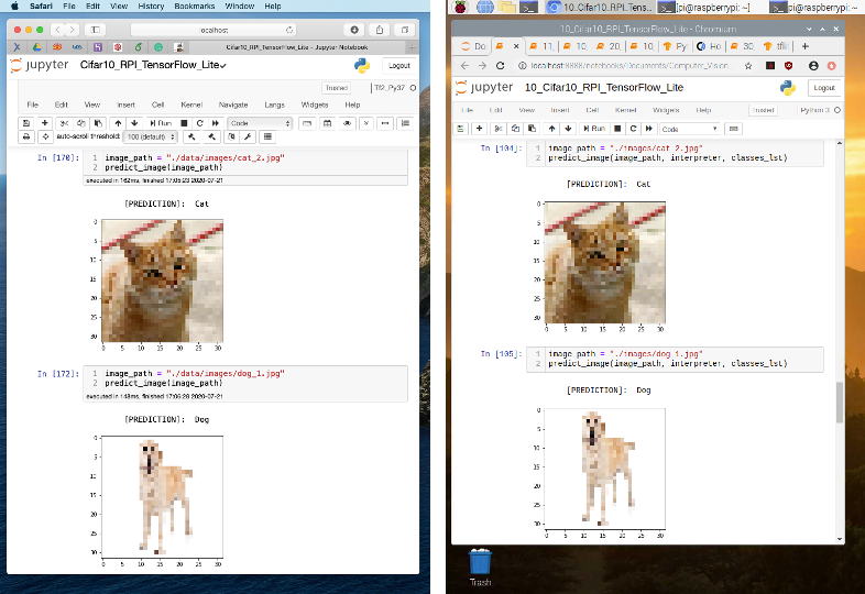
The figure below shows some tests using the function:

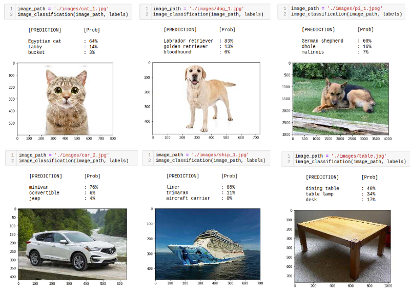
The overall performance is astonishing! From the instant that you enter with the image path in the memory card, until the time that that result is printed out, all process took less than half a second, with high precision!

The function can be easily applied to frames on videos or live camera. The notebook for that and the complete code discussed in this section can be downloaded from GitHub.

Object Detection

With Image Classification, we can detect what the dominant subject of such an image is. But what happens if several objects are dominant and of interest on the same image? To solve it, we can use an Object Detection model!

Given an image or a video stream, an object detection model can identify which of a known set of objects might be present and provide information about their positions within the image.

For this task, we will download a Mobilenet V1 model pre-trained using the COCO (Common Objects in Context) dataset. This dataset has more than 200,000 labeled images, in 91 categories.

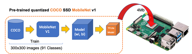
Downloading model and labels

On Raspberry terminal run the commands:

$ cd ./models 
$ curl -O http://storage.googleapis.com/download.tensorflow.org/models/tflite/coco_ssd_mobilenet_v1_1.0_quant_2018_06_29.zip
$ unzip coco_ssd_mobilenet_v1_1.0_quant_2018_06_29.zip
$ curl -O  https://dl.google.com/coral/canned_models/coco_labels.txt

$ rm coco_ssd_mobilenet_v1_1.0_quant_2018_06_29.zip
$ rm labelmap.txt

On models subdirectory, we should end with 2 new files:

coco_labels.txt  
detect.tflite

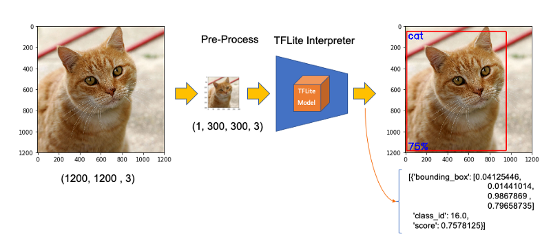
The steps to perform inference on a new image, are very similar to those done with Image Classification, except that:

• input: image must have a shape of 300×300 pixels
• output: include not only label and probability (“score”), but also the relative window position (“ Bounding Box”) about where the object is located on the image.

Now, we must load the labels and model, allocating tensors. 

labels = load_labels('./models/coco_labels.txt')
interpreter = Interpreter('./models/detect.tflite')
interpreter.allocate_tensors()

The input pre-process is the same as we did before, but the output should be worked to get a more readable output. The functions below will help with that:

def set_input_tensor(interpreter, image):
    """Sets the input tensor."""
    tensor_index = interpreter.get_input_details()[0]['index']
    input_tensor = interpreter.tensor(tensor_index)()[0]
    input_tensor[:, :] = image

def get_output_tensor(interpreter, index):
    """Returns the output tensor at the given index."""
    output_details = interpreter.get_output_details()[index]
    tensor = np.squeeze(interpreter.get_tensor(output_details['index']))
    return tensor

With the help of the above functions, detect_objects() will return the inference results:

• object label id
• score
• the bounding box, that will show where the object is located.

We have included a ‘threshold’ to avoid objects with a low probability of being correct. Usually, we should consider a score above 50%.

def detect_objects(interpreter, image, threshold):
    set_input_tensor(interpreter, image)
    interpreter.invoke()
    
    # Get all output details
    boxes = get_output_tensor(interpreter, 0)
    classes = get_output_tensor(interpreter, 1)
    scores = get_output_tensor(interpreter, 2)
    count = int(get_output_tensor(interpreter, 3))

    results = []
    for i in range(count):
        if scores[i] >= threshold:
            result = {
                'bounding_box': boxes[i],
                'class_id': classes[i],
                'score': scores[i]
            }
            results.append(result)
    return results

If we apply the above function to a reshaped image (same as used on classification example), we should get:

Great! In less than 200ms with 77% probability, an object with id 16 was detected on an area delimited by a ‘bounding box’: (0.028011084, 0.020121813, 0.9886069, 0.802299). Those four numbers are respectively related to ymin, xmin, ymax and xmax.

Take into consideration that y goes from the top (ymin) to bottom (ymax) and x goes from left (xmin) to the right (xmax) as shown in figure below:

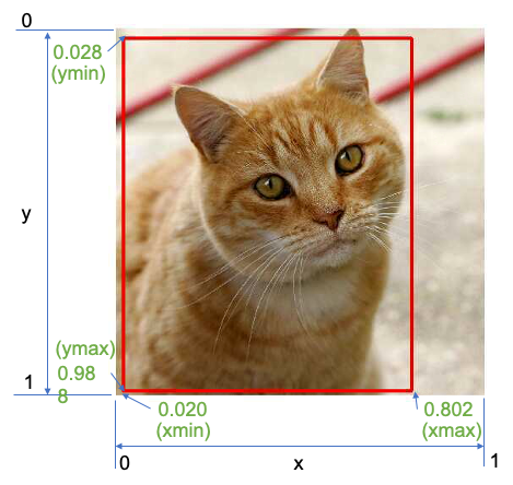
Having the bounding box four values, we have, in fact, the coordinates of the top/left corner and the bottom/right one. With both edges and knowing the shape of the picture, it is possible to draw the rectangle around the object.

Next, we should find what class_id equal to 16 means. Opening the file coco_labels.txt, as a dictionary, each of its elements has an index associated, and inspecting index 16, we get as expected, ‘cat.’ The probability is the value returning from the score.

Let’s create a general function to detect multiple objects on a single picture. The first function, starting from an image path, will execute the inference, returning the resized image and the results (multiples ids, each one with its scores and bounding boxes:

def detectObjImg_2(image_path, threshold = 0.51):

img = cv2.imread(image_path)
    img = cv2.cvtColor(img, cv2.COLOR_BGR2RGB)
    image = cv2.resize(img, (width, height),
                       fx=0.5,
                       fy=0.5,
                       interpolation=cv2.INTER_AREA)
    results = detect_objects(interpreter, image, threshold)

return img, results

Having the reshaped image, and inference results, the below function can be used to draw a rectangle around the objects, specifying for each one, its label and probability:

def detect_mult_object_picture(img, results):

    HEIGHT, WIDTH, _ = img.shape
    aspect = WIDTH / HEIGHT
    WIDTH = 640
    HEIGHT = int(640 / aspect)
    dim = (WIDTH, HEIGHT)

   img = cv2.resize(img, dim, interpolation=cv2.INTER_AREA)

   for i in range(len(results)):
        id = int(results[i]['class_id'])
        prob = int(round(results[i]['score'], 2) * 100)
        
        ymin, xmin, ymax, xmax = results[i]['bounding_box']
        xmin = int(xmin * WIDTH)
        xmax = int(xmax * WIDTH)
        ymin = int(ymin * HEIGHT)
        ymax = int(ymax * HEIGHT)

        text = "{}: {}%".format(labels[id], prob)

        if ymin > 10: ytxt = ymin - 10
        else: ytxt = ymin + 15

        img = cv2.rectangle(img, (xmin, ymin), (xmax, ymax),
                            COLORS[id],
                            thickness=2)
        img = cv2.putText(img, text, (xmin + 3, ytxt), FONT, 0.5, COLORS[id],
                          2)

   return img

Below some results:

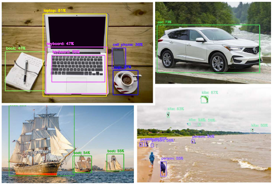
The complete code can be found at GitHub.

Object Detection using Camera

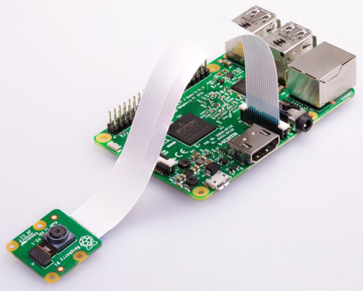
If you have a PiCam connected to Raspberry Pi, it is possible to capture a video and perform object recognition, frame by frame, using the same functions defined before. Please follow this tutorial if you do not have a working camera in your Pi: Getting started with the Camera Module.

First, it is essential to define the size of the frame to be captured by the camera. We will use 640×480.

WIDTH = 640
HEIGHT = 480

Next, you must iniciate the camera:

cap = cv2.VideoCapture(0)
cap.set(3, WIDTH)
cap.set(4, HEIGHT)

And run the below code in a loop. Until the key ‘q’ is pressed, the camera will capture the video, frame by frame, drawing the bounding box with its respective labels and probabilities.

while True:

    timer = cv2.getTickCount()
    success, img = cap.read()
    img = cv2.flip(img, 0)
    img = cv2.flip(img, 1)

    fps = cv2.getTickFrequency() / (cv2.getTickCount() - timer)
    cv2.putText(img, "FPS: " + str(int(fps)), (10, 470),
                cv2.FONT_HERSHEY_SIMPLEX, 0.7, (0, 0, 255), 2)

    image = cv2.cvtColor(img, cv2.COLOR_BGR2RGB)
    image = cv2.resize(image, (width, height),
                       fx=0.5,
                       fy=0.5,
                       interpolation=cv2.INTER_AREA)
    start_time = time.time()
    results = detect_objects(interpreter, image, 0.55)
    elapsed_ms = (time.time() - start_time) * 1000

    img = detect_mult_object_picture(img, results)
    cv2.imshow("Image Recognition ==> Press [q] to Exit", img)

if cv2.waitKey(1) & 0xFF == ord('q'):
        break

cap.release()
cv2.destroyAllWindows()

Below is possible to see the video running in real-time on the Raspberry Pi screen. Note that the video runs around 60 FPS (frames per second), which is pretty good!

Here one screen-shot of the above video:

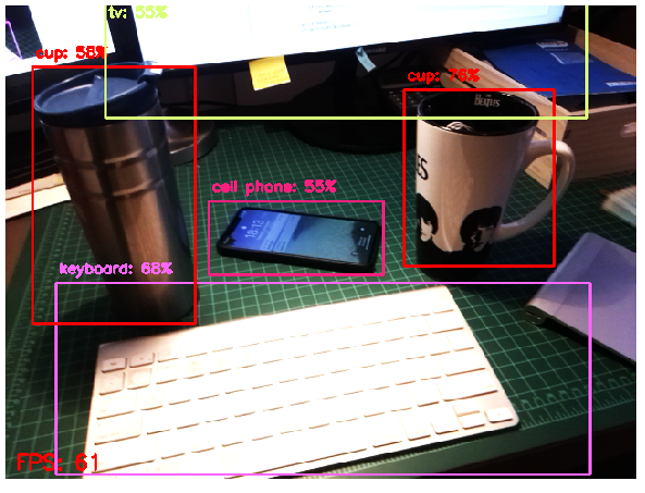
The complete code is available on GitHub. 

Pose Estimation

One of the more exciting and critical areas of AI is to estimate a person’s real-time pose, enabling machines to understand what people are doing in images and videos. Pose estimation was deeply explored in my article Realtime Multiple Person 2D Pose Estimation using TensorFlow2.x, but here at the Edge, with a Raspberry Pi and with the help of TensorFlow Lite, it is possible to easily replicate almost the same that was done on a Mac.

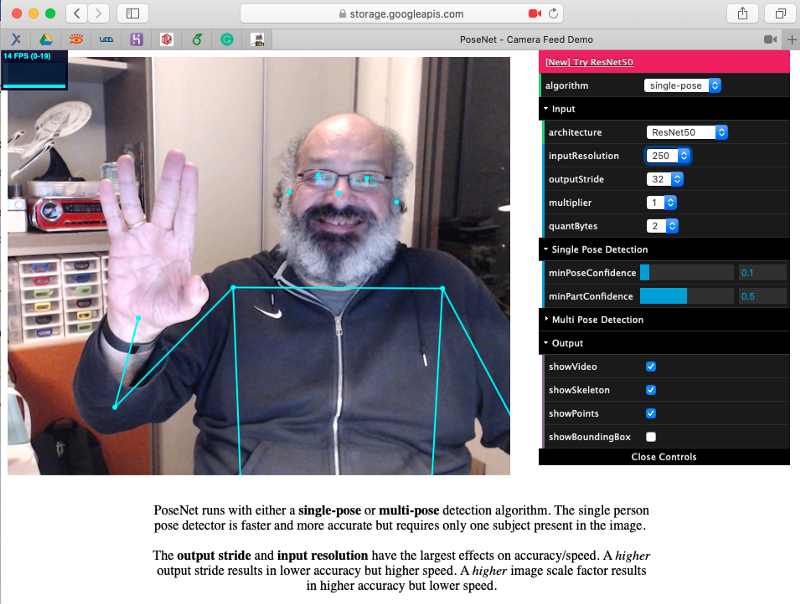
The model that we will use in this project is the PoseNet. We will do inference the same way done for Image Classification and Object Detection, where an image is fed through a pre-trained model. PoseNet comes with a few different versions of the model, corresponding to variances of MobileNet v1 architecture and ResNet50 architecture. In this project, the version pre-trained is the MobileNet V1, which is smaller, faster, but less accurate than ResNet. Also, there are separate models for single and multiple person pose detection. We will explore the model trained for a single person.

In this site is possible to explore in real time and using a live camera, several PoseNet models and configurations.

The libraries to execute Pose Estimation on a Raspberry Pi are the same used before. NumPy, MatPlotLib, OpenCV and TensorFlow Lite Interpreter.

The pre-trained model is the posenet_mobilenet_v1_100_257x257_multi_kpt_stripped.tflite, which can be downloaded from the above link or the TensorFlow Lite — Pose Estimation Overview website. The model should be saved in the models subdirectory.

Start loading TFLite model and allocating tensors:

interpreter = tflite.Interpreter(model_path='./models/posenet_mobilenet_v1_100_257x257_multi_kpt_stripped.tflite')
interpreter.allocate_tensors()

Get input and output tensors:

input_details = interpreter.get_input_details()
output_details = interpreter.get_output_details()

Same as we did before, looking into the input_details, it is possible to see that the image to be used to pose estimation should be (1, 257, 257, 3), which means that images must be reshaped to 257×257 pixels.

Let’s take as input a simple human figure, that will help us to analyze it:

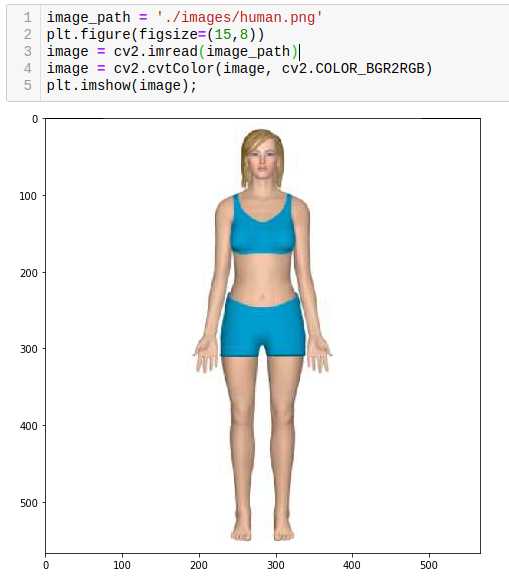
The first step is to pre-process the image. This particular model was not quantized, which means that the dtype is float32. This information is essential to pre-process the input image, as shown with the below code

image = cv2.resize(image, size) 
input_data = np.expand_dims(image, axis=0)
input_data = input_data.astype(np.float32)
input_data = (np.float32(input_data) - 127.5) / 127.5

Having the image pre-processed, now it is time to perform the inference, feeding the tensor with the image and invoking the interpreter:

interpreter.set_tensor(input_details[0]['index'], input_data)
interpreter.invoke()

An article that helps a lot to understand how to work with PoseNet is the Ivan Kunyakin tutorial’s Pose estimation and matching with TensorFlow lite. There Ivan comments that on the output vector, what matters to find the key points, are:

• Heatmaps 3D tensor of size (9,9,17), that corresponds to the probability of appearance of each one of the 17 keypoints (body joints) in the particular part of the image (9,9). It is used to locate the approximate position of the joint.
• Offset Vectors: 3D tensor of size (9,9,34) that is called offset vectors. It is used for more exact calculation of the keypoint’s position. The First 17 of the third dimension correspond to the x coordinates and the second 17 of them to the y coordinates.

output_details = interpreter.get_output_details()[0]
heatmaps = np.squeeze(interpreter.get_tensor(output_details['index']))

output_details = interpreter.get_output_details()[1]
offsets = np.squeeze(interpreter.get_tensor(output_details['index']))

Let’s create a function that will return an array with all 17 keypoints (or person’s joints) based on heatmaps and offsets.

def get_keypoints(heatmaps, offsets):

    joint_num = heatmaps.shape[-1]
    pose_kps = np.zeros((joint_num, 2), np.uint32)
    max_prob = np.zeros((joint_num, 1))

    for i in range(joint_num):
        joint_heatmap = heatmaps[:,:,i]
        max_val_pos = np.squeeze(
            np.argwhere(joint_heatmap == np.max(joint_heatmap)))
        remap_pos = np.array(max_val_pos / 8 * 257, dtype=np.int32)
        pose_kps[i, 0] = int(remap_pos[0] +
                             offsets[max_val_pos[0], max_val_pos[1], i])
        pose_kps[i, 1] = int(remap_pos[1] +
                             offsets[max_val_pos[0], max_val_pos[1],
                                         i + joint_num])
        max_prob[i] = np.amax(joint_heatmap)

    return pose_kps, max_prob

Using the above function with the heatmaps and offset vectors that were extracted from the output tensor, resultant of the image inference, we get:

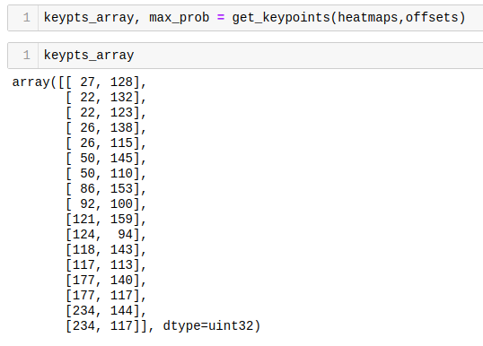
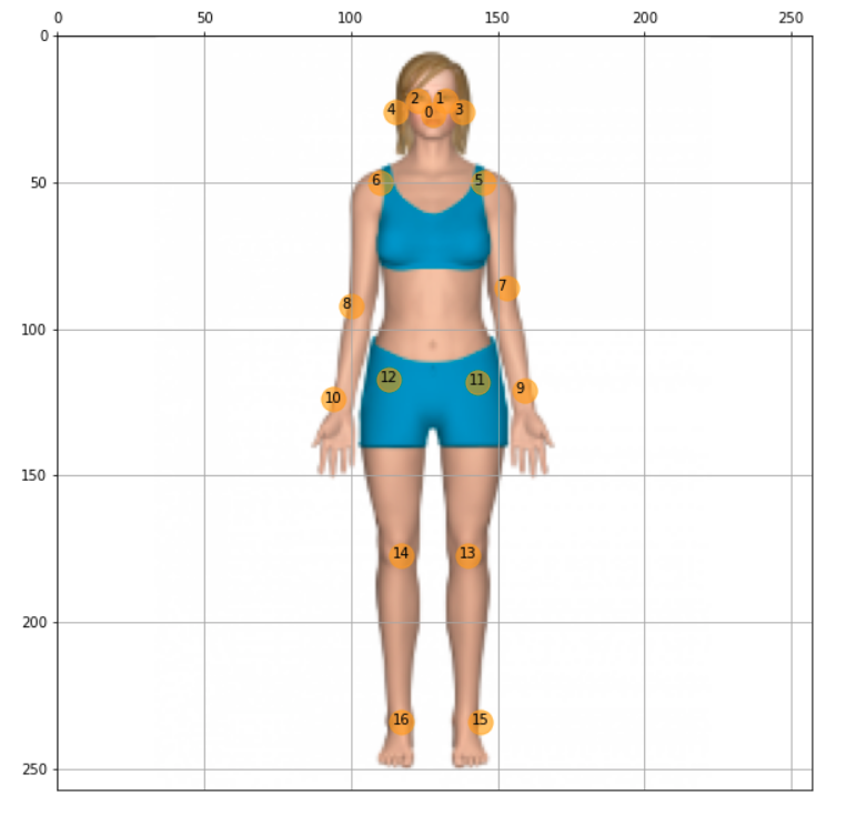
The resultant array shows all 17 coordinates (y, x) regarding where the joints are located on an image of 257 x 257 pixels. Using the code below. It is possible to plot each one of the joints over the resized image. For reference, the array index is annotated, so it is easy to identify each joint:

y,x = zip(*keypts_array)
plt.figure(figsize=(10,10))
plt.axis([0, image.shape[1], 0, image.shape[0]])  
plt.scatter(x,y, s=300, color='orange', alpha=0.6)
img = cv2.cvtColor(image, cv2.COLOR_BGR2RGB)
plt.imshow(img)
ax=plt.gca() 
ax.set_ylim(ax.get_ylim()[::-1]) 
ax.xaxis.tick_top() 
plt.grid();

for i, txt in enumerate(keypts_array):
    ax.annotate(i, (keypts_array[i][1]-3, keypts_array[i][0]+1))

As a result, we get the picure:

Great, now it is time to create a general function to draw “the bones”, which is the joints’ connection. The bones will be drawn as lines, which are the connections among keypoints 5 to 16, as shown in the above figure. Independent circles will be used for keypoints 0 to 4, related to head:

def join_point(img, kps, color='white', bone_size=1):
    
    if   color == 'blue'  : color=(255, 0, 0)
    elif color == 'green': color=(0, 255, 0)
    elif color == 'red':  color=(0, 0, 255)
    elif color == 'white': color=(255, 255, 255)
    else:                  color=(0, 0, 0)

    body_parts = [(5, 6), (5, 7), (6, 8), (7, 9), (8, 10), (11, 12), (5, 11),
                  (6, 12), (11, 13), (12, 14), (13, 15), (14, 16)]

    for part in body_parts:
        cv2.line(img, (kps[part[0]][1], kps[part[0]][0]),
                (kps[part[1]][1], kps[part[1]][0]),
                color=color,
                lineType=cv2.LINE_AA,
                thickness=bone_size)
    
    for i in range(0,len(kps)):
        cv2.circle(img,(kps[i,1],kps[i,0]),2,(255,0,0),-1)

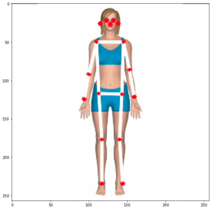
Calling the function, we have the estimated pose of the body in the image:

join_point(img, keypts_array, bone_size=2)
plt.figure(figsize=(10,10))
plt.imshow(img);

And last but not least, let’s create a general function to estimate posture having an image path as a start:

def plot_pose(img, keypts_array, joint_color='red', bone_color='blue', bone_size=1):
    join_point(img, keypts_array, bone_color, bone_size)
    y,x = zip(*keypts_array)
    plt.figure(figsize=(10,10))
    plt.axis([0, img.shape[1], 0, img.shape[0]])  
    plt.scatter(x,y, s=100, color=joint_color)
    img = cv2.cvtColor(img, cv2.COLOR_BGR2RGB)

    plt.imshow(img)
    ax=plt.gca() 
    ax.set_ylim(ax.get_ylim()[::-1]) 
    ax.xaxis.tick_top() 
    plt.grid();
    return img

def get_plot_pose(image_path, size, joint_color='red', bone_color='blue', bone_size=1):    
    image_original = cv2.imread(image_path)
    image = cv2.resize(image_original, size) 
    input_data = np.expand_dims(image, axis=0)
    input_data = input_data.astype(np.float32)
    input_data = (np.float32(input_data) - 127.5) / 127.5

    interpreter.set_tensor(input_details[0]['index'], input_data)
    interpreter.invoke()
    
    output_details = interpreter.get_output_details()[0]
    heatmaps = np.squeeze(interpreter.get_tensor(output_details['index']))

    output_details = interpreter.get_output_details()[1]
    offsets = np.squeeze(interpreter.get_tensor(output_details['index']))

    keypts_array, max_prob = get_keypoints(heatmaps,offsets)
    orig_kps = get_original_pose_keypoints(image_original, keypts_array, size)

    img = plot_pose(image_original, orig_kps, joint_color, bone_color, bone_size)
    
    return orig_kps, max_prob, img

At this point with only one line of code, it is possible to detect pose on images:

keypts_array, max_prob, img  = get_plot_pose(image_path, size, bone_size=3)

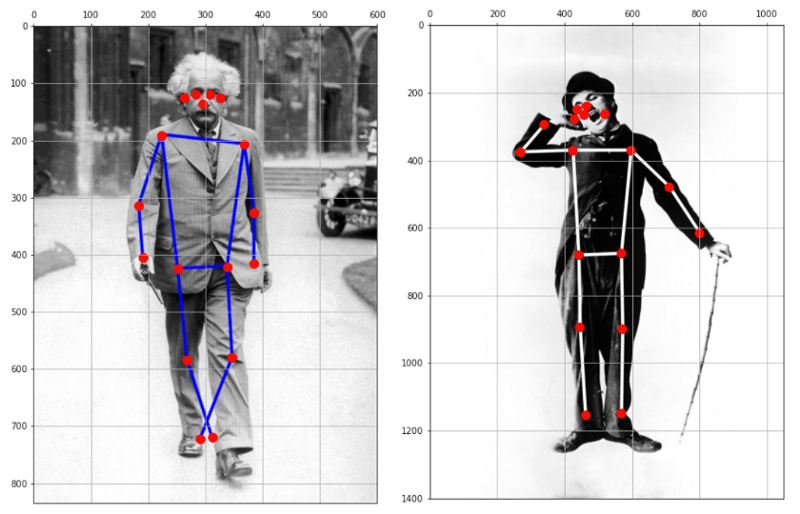
All code developed on this section is available on GitHub. 

Another easy step is to apply the function to frames from videos and live camera. I will leave it for you! 😉

Conclusion

TensorFlow Lite is a great framework to implement Artificial Intelligence (more precisely, ML) at the Edge. Here we explored ML models working on a Raspberry Pi, but TFLite is now more and more used at the “edge of the edge”, on very small microcontrollers, in what has been called TinyML. 

As always, I hope this article can inspire others to find their way in the fantastic world of AI!

All the codes used in this article are available for download on project GitHub: TFLite_IA_at_the_Edge.

Regards from the South of the World!

See you in my next article!

Thank you

Marcelo