Sensing the Air Quality

A low-cost IoT Air Quality Monitor based on RaspberryPi 4

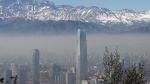
I have the privilege of living in one of the most beautiful countries in the world, but unfortunately, it’s not all roses. Chile during winter season suffers a lot with air contamination, mainly due to particulate materials as dust and smog.

Because of cold weather, in the south, air contamination is mainly due to wood-based calefactors and in Santiago (the main capital in the center of the country) mixed from industries, cars, and its unique geographic situation between 2 huge mountains chains.

 

Nowadays, air pollution is a big problem all over the world and in this article we will explore how to develop a low expensive homemade Air Quality Station, based on a Raspberry Pi.

If you are interested to understand more about it,  please visit the “World Air Quality Index” Project.

The particulate matter (PM), what is, and how does it get into the air?

So, to understand pollution or air contamination, we must study the particles that are related to that, that are the particulate matter. Looking at the graphs on the previous section we can observe that they mentioned PM2.5 and PM10. Let’s give a quick overview of that.

PM stands for particulate matter (also called particle pollution): the term for a mixture of solid particles and liquid droplets found in the air. Some particles, such as dust, dirt, soot, or smoke, are large or dark enough to be seen with the naked eye. Others are so small they can only be detected using an electron microscope.

Particles come in a wide range of sizes. Particles less than or equal to 10 micrometers in diameter are so small that they can get into the lungs, potentially causing serious health problems. Ten micrometers is less than the width of a single human hair.

Particle pollution includes:

• Coarse dust particles (PM_{10 )}: inhalable particles, with diameters that are generally 10 micrometers and smaller. Sources include crushing or grinding operations and dust stirred up by vehicles on roads.
• Fine particles (PM_2.5): fine inhalable particles, with diameters that are generally 2.5 micrometers and smaller. Fine particles are produced from all types of combustion, including motor vehicles, power plants, residential wood burning, forest fires, agricultural burning, and some industrial processes

You can find more about particulate matter on EPA site: United States Environmental Protection Agency

Why is important care about those particulate matters? 

As described by GERARDO ALVARADO Z. in his work, studies of episodes of high air pollution in the Meuse Valley (Belgium) in 1930, Donora (Pennsylvania) in 1948 and London in 1952 have been the first documented sources that related mortality with particle contamination (Préndez, 1993). Advances in the investigation of the effects of air pollution on people’s health have determined that health risks are caused by inhalable particles, depending on their penetration and deposition in different sections of the respiratory system, and the Biological response to deposited materials.

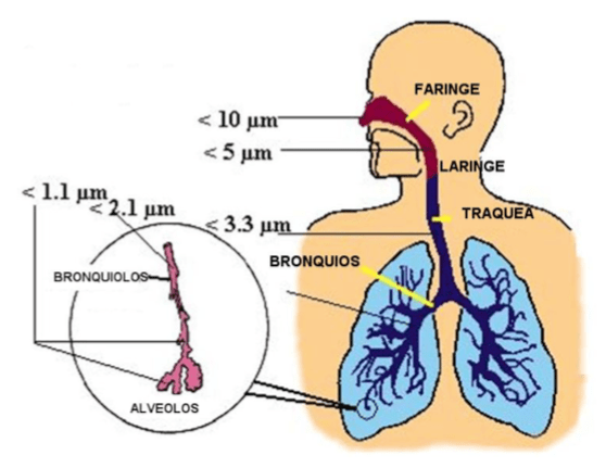
The thickest particles, about 5 μm, are filtered by the joint action of the cilia of the nasal passage and the mucosa that covers the nasal cavity and the trachea. Particles with a diameter between 0.5 and 5 μm can be deposited in the bronchi and even in the pulmonary alveoli, however, they are eliminated by the cilia of bronchi and bronchioles after a few hours. Particles smaller than 0.5 μm can penetrate deeply until they are deposited in the pulmonary alveoli, remaining from weeks to years, since there is no mucociliary transport mechanism that facilitates elimination.

The following figure shows the penetration of the particles in the respiratory system depending on their size.

So, to spot both types of particles (PM2.5 and PM10) are very important and the good news is that both are readable by a simple and not expensive sensor, the SDS011.

The Particle Sensor – SDS011

Air Quality monitoring is well known and established science which started back in the 80’s. At that time, the technology was quite limited, and the solution used to quantify the air pollution complex, cumbersome and really expensive.

Fortunately, nowadays, with the most recent and modern technologies, the solutions used for Air Quality monitoring are becoming not only more precise but also faster at measuring. Devices are becoming smaller, and cost much more affordable than ever before.

In this article we will focus on a particle sensor, that can detect the amount of dust in the air. While the first generation was just able to detect the amount of opacity, most recent sensors as the SDS011 from INOVAFIT, a spin-off from the University of Jinan (in Shandong), can now detect PM2.5 and PM10.

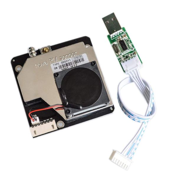
With its size, the SDS011 is probably one of the best sensors in terms of accuracy and price (less than $40.00).

Specifications

• Measured values: PM2.5, PM10
• Range: 0 – 999.9 μg /m³
• Supply voltage: 5V (4.7 – 5.3V)
• Power consumption (work): 70mA±10mA
• Power consumption (sleep mode laser & fan): < 4mA
• Storage temperature: -20 to +60C
• Work temperature: -10 to +50C
• Humidity (storage): Max. 90%
• Humidity (work): Max. 70% (condensation of water vapor falsify readings)
• Accuracy:
  • 70% for 0.3μm
  • 98% for 0.5μm
• Size: 71x70x23 mm
• Certification: CE, FCC, RoHS

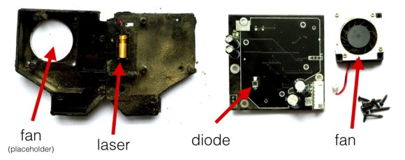
The SD011 use the PCB as one side of the casing (allowing to reduce the cost). The diode is mounted on the PCB side (this is mandatory as any noise between the diode and the LNA should be avoided). The laser mounted on the plastic box and connected to the PCB via a flying wire.

In short, Nova Fitness SDS011 is a professional laser dust sensor. Fan mounted on sensor automatically sucks air. The sensor uses a laser light scattering principle* to measure the value of dust particles suspended in the air. The sensor provides high precision and reliable readings of PM2.5 and PM10 values. Any change in environment can be observed almost instantaneously – short respond time below 10 seconds. The sensor in standard mode reports reading with a 1-second interval.

* Laser Scattering Principle: Light scattering can be induced when particles go through the detecting area. The scattered light is transformed into electrical signals and these signals will be amplified and processed. The number and diameter of particles can be obtained by analysis because the signal waveform has certain relations with the particles diameter. 

 But how the SDS011 can capture those particles?

As commented before, the principle used by SDS011 is light scattering or better Dynamic Light Scattering (DLS), that is a technique in physics that can be used to determine the size distribution profile of small particles in suspension or polymers in solution. In the scope of DLS, temporal fluctuations are usually analyzed by means of the intensity or photon auto-correlation function (also known as photon correlation spectroscopy or quasi-elastic light scattering). In the time domain analysis, the autocorrelation function (ACF) usually decays starting from zero delay time, and faster dynamics due to smaller particles lead to faster decorrelation of scattered intensity trace. It has been shown that the intensity ACF is the Fourier transform of the power spectrum, and therefore the DLS measurements can be equally well performed in the spectral domain.

Below a hypothetical dynamic light scattering of two samples: Larger particles (like PM10) on the top and smaller particles (as PM2.5) on the bottom:

And looking inside our sensor, we can see how the light scatter principle is implemented:

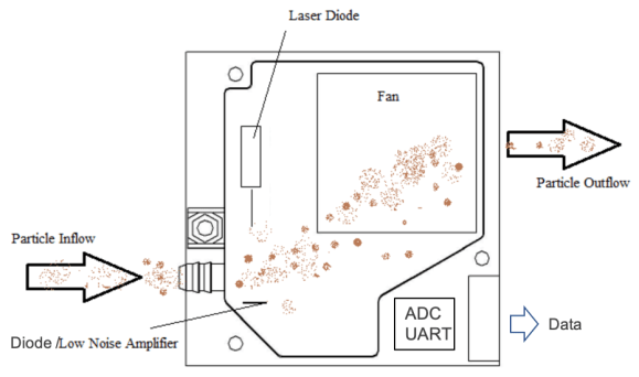
The electrical signal captured on the diode goes to Low Noise Amplifier and from that to be converted to digital signal thru an ADC and to outside via an UART.

To know more about SDS011 on a real scientific experience, please take a look on the 2018 work of Konstantinos et all, Development and On-Field Testing of Low-Cost Portable System for Monitoring PM2.5 Concentrations.

Showtime!

Let’s take a break on all this theory and focus on how to measure particulate matters using a Raspberry Pi and the SOS011 sensor

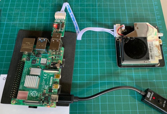
The HW connection is in fact very simple. The sensor is sold with a USB adapter to interface the output data from its 7 pins UART with one of the RPi’s standard USB connector.

SDS011 pinout:

• Pin 1 – not connected
• Pin 2 – PM2.5: 0-999μg/m³; PWM output
• Pin 3 – 5V
• Pin 4 – PM10: 0-999 μg/m³; PWM output
• Pin 5 – GND
• Pin 6 – RX UART (TTL) 3.3V
• Pin 7 – TX UART (TTL) 3.3V

For this tutorial, I am using for the first time a brand new Raspberry-Pi 4. But of course, any previous model will also work fine.

As soon you connect the sensor on one of the RPi USB ports, you automatically will start to listen to the sound of its fan. The noise is a little bit annoying, so maybe you should unplug it and wait until you have all set with SW.

The communication between sensor and RPi will be thru a serial protocol. Details about this protocol can be found here: Laser Dust Sensor Control Protocol V1.3.

But for this project, the best is to use a python interface to simplify the code to be developed. You can create your own interface or use some that are available on the internet, as Frank Heuer‘s or Ivan Kalchev’s. We will use the last one, that is very simple and works fine (you can download the sds011.py script from its GitHub or mine).

The file sds011.py must be at same directory where you create your script.

During the development phase, I will use a Jupyter Notebook, but you can use any IDE that you like (Thonny or Geany, for example, that are part of Raspberry Pi Debian package are both very good).

Plug your sensor on one of the USBs. Once only one USB is being used, the serial port on your RPI should be: /dev/ttyUSB0. 

Start importing sds011, and creating your sensor instance. SDS011 provides a method to read from the sensor using a UART.

from sds011 import *
sensor = SDS011("/dev/ttyUSB0")

You can turn on or off your sensor with the command sleep:

# Turn-on sensor
sensor.sleep(sleep=False)

# Turn-off sensor
sensor.sleep(sleep=True)

Once the sensor is turned on (wait at least 10 seconds for stabilization),  you can get data from the sensor using:

pmt_2_5, pmt_10 = sensor.query()

Wait at least 10 seconds for stabilization before measurements and at least 2 seconds to start a new one:

And this is all you need to know in terms of SW to use the sensor. But let’s go deeper on Air Quality Control! At the beginning of this article, if you have explored the sites that give information about how good or bad is the air, you should realize that colors are associated with those values. Each color is an Index. The most known of that is the AQI (Air Quality Index), used in the US and several other countries.

Air Quality Index — AQI

The AQI is an index for reporting daily air quality. It tells you how clean or polluted your air is, and what associated health effects might be a concern for you. The AQI focuses on health effects you may experience within a few hours or days after breathing polluted air.

EPA (the United States Environmental Protection Agency), for example, calculates the AQI not only for particle pollution (PM2.5 and PM10) but also for the other major air pollutants regulated by the Clean Air Act: ground-level ozone, carbon monoxide, sulfur dioxide, and nitrogen dioxide. For each of these pollutants, EPA has established national air quality standards to protect public health.

AQI values, colors and health message associated:

As commented before those AQI values and colors are related with each one of pollutant agents, but how to associate the values generated by sensors with them?

An additional table connects them all:

But of course, makes no sense take use of such table. In the end, it is a simple mathematical algorithm that makes the calculation. For that, we will import the library to convert between AQI value and pollutant concentration (µg/m³):
python-aqi.

Install the library using PIP:

pip install python-aqi

And how about Chile?

In Chile a similar index is used, the ICAP: Air Quality Index for Breathable Particles. A Supreme Decree 59 of March 16, 1998, of the General Secretary Ministry of the Presidency of the Republic, establishes in its article 1, letter g) that the levels that define the ICA for Breathable Particulate Material, ICAP, are those that show in the following table:

The values will vary linearly between the sections, the value 500 would correspond to the limit value over which there would be a risk for the population when exposed to these concentrations. According to the ICAP values, categories were established (see Table below) that qualify the concentration levels of MP10 to which people were exposed:

Logging Data Locally

At this point, we can have all the tools to capture data from the sensor and also converted them for a more “readable value”, that it is the AQI index.

Let’s create a function to capture those values. We will capture 3 values in sequence taking the average among them:

def get_data(n=3):
    sensor.sleep(sleep=False)
    pmt_2_5 = 0
    pmt_10 = 0
    time.sleep(10)
    for i in range (n):
        x = sensor.query()
        pmt_2_5 = pmt_2_5 + x[0]
        pmt_10 = pmt_10 + x[1]
        time.sleep(2)
    pmt_2_5 = round(pmt_2_5/n, 1)
    pmt_10 = round(pmt_10/n, 1)
    sensor.sleep(sleep=True)
    time.sleep(2)
    return pmt_2_5, pmt_10

Let’s test it:

Ben Orlin — MathWithBadDrawings

Let’s also do a function to convert the numeric values of PM in AQI index:

def conv_aqi(pmt_2_5, pmt_10):
    aqi_2_5 = aqi.to_iaqi(aqi.POLLUTANT_PM25, str(pmt_2_5))
    aqi_10 = aqi.to_iaqi(aqi.POLLUTANT_PM10, str(pmt_10))
    return aqi_2_5, aqi_10

And test both functions together:

But what to do with them?

The most simple answer is to create a function to save the captured data, saving them on a local file:

def save_log(): 
    with open("YOUR PATH HERE/air_quality.csv", "a") as log:
    dt = datetime.now()
    log.write("{},{},{},{},{}\n".format(dt, pmt_2_5, aqi_2_5,       pmt_10,aqi_10))
    log.close()

With a single loop, you can log data at regular bases in your local file, for example, each minute:

while(True): 
    pmt_2_5, pmt_10 = get_data()
    aqi_2_5, aqi_10 = conv_aqi(pmt_2_5, pmt_10)
    try:
        save_log()
    except:
        print ("[INFO] Failure in logging data") 
    time.sleep(60)

Every 60 seconds, the timestamp plus the data will be “append” to this file, as we can see above.

Sending Data to a Cloud Service

At this point, we have learned how to capture data from the sensor, saving them on a local CSV file. Now, it is time to see how to send those data to an IoT platform. On this tutorial, we will use ThingSpeak.com.

“ThingSpeak is an open source Internet of Things (IoT) application to store and retrieve data from things, using REST and MQTT APIs. ThingSpeak enables the creation of sensor logging applications, location tracking applications, and a social network of things with status updates.”

First, you must have an account at ThinkSpeak.com. Next, follow the instructions to create a Channel, taking note of its Channel ID and Write API Key.

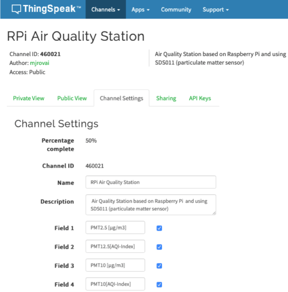
When creating the channel, you must also define what info will be uploaded to each one of the 8 fields, as shown above (in our case only 4 of them will be used).

MQTT Protocol and ThingSpeak Connection

MQTT is a publish/subscribe architecture that was developed primarily to connect bandwidth and power-constrained devices over wireless networks. It is a simple and lightweight protocol that runs over TCP/IP sockets or WebSockets. MQTT over WebSockets can be secured with SSL. The publish/subscribe architecture enables messages to be pushed to the client devices without the device needing to continuously poll the server.

The MQTT broker is the central point of communication, and it is in charge of dispatching all messages between the senders and the rightful receivers. A client is any device that connects to the broker and can publish or subscribe to topics to access the information. A topic contains routing information for the broker. Each client that wants to send messages publishes them to a certain topic, and each client that wants to receive messages subscribes to a certain topic. The broker delivers all messages with the matching topic to the appropriate clients.

ThingSpeak™ has an MQTT broker at the URL mqtt.thingspeak.com and port 1883. The ThingSpeak broker supports both MQTT publish and MQTT subscribe.

In our case, we will use the MQTT Publish.

MQTT Publish

For starting, let’s install the Eclipse Paho MQTT Python client library, that implements versions 3.1 and 3.1.1 of the MQTT protocol

sudo pip install paho-mqtt

Next, let’s import the paho library:

import paho.mqtt.publish as publish

and initiate the Thingspeak channel and MQTT protocol. This connection method is the simplest and requires the least system resources:

channelID = "YOUR CHANNEL ID"
apiKey = "YOUR WRITE KEY"
topic = "channels/" + channelID + "/publish/" + apiKey
mqttHost = "mqtt.thingspeak.com"

Now we must define our “payload”:

tPayload = "field1=" + str(pmt_2_5)+ "&field2=" + str(aqi_2_5)+ "&field3=" + str(pmt_10)+ "&field4=" + str(aqi_10)

And that’s it! we are ready to start sending data to the cloud!

Let’s rewrite the previous loop function to also include the ThingSpeak part of it.

# Sending all data to ThingSpeak every 1 minute
while(True): 
    pmt_2_5, pmt_10 = get_data()
    aqi_2_5, aqi_10 = conv_aqi(pmt_2_5, pmt_10)
    tPayload = "field1=" + str(pmt_2_5)+ "&field2=" + str(aqi_2_5)+ "&field3=" + str(pmt_10)+ "&field4=" + str(aqi_10)
    try:
        publish.single(topic, payload=tPayload, hostname=mqttHost, port=tPort, tls=tTLS, transport=tTransport)
        save_log()
    except:
        print ("[INFO] Failure in sending data") 
    time.sleep(60)

If everything is ok, you must see data also appear on your channel at thingspeak.com:

The Final Script

It is important to point that Jupyter Notebook is a very good tool for development and report, but no to create a code to put in production. What you should do now is take the relevant part of the code and create a .py script and run it on your terminal.

For example, “ts_air_quality_logger.py”, that you should run with the command:

python 3 ts_air_quality_logger.py

This script as well the Jupyter Notebook and the sds011.py can be found in my repository at RPi_Air_Quality_Sensor.

Note that this script is feasible for testing only. The best is not to use delays inside the final loop (that put the code in “pause”), instead use timers. Or for a real application, the best is not use the loop, having the Linux programed to executed the script at regular basis with crontab.

Testing the monitor

Once my Raspberry Pi Air Quality monitor was working, I assembled the RPi inside a plastic box, keeping the sensor outside and placed it outside my home.

Two experiences were made:

1. Gasoline Motor Combustion: The sensor was placed around 1m from the Lambretta’s gas scape, and its motor turned on:

I left the motor running for a couple of minutes and turned off. From log file, this is the result that I got:

Interesting to confirm that PM2.5 was the most dangerous particulate that resulted from the motor.

2. Wood Burning: the wood fire was placed directly under the nose:

Looking at the log file:

The sensor data was momentaneous “out of Range” and was not well captured by AQI conversion Library, so I change previous code to handle it:

def conv_aqi(pmt_2_5, pmt_10):
    try:
        aqi_2_5 = aqi.to_iaqi(aqi.POLLUTANT_PM25, str(pmt_2_5))
        aqi_10 = aqi.to_iaqi(aqi.POLLUTANT_PM10, str(pmt_10))
        return aqi_2_5, aqi_10
    except:
        return 600, 600

This situation can happen in the field, which is OK. Remember that in fact, you should use moving average to really get the AQI (hourly at least, but usually daily).

Conclusion

As always, I hope this project can help others find their way into the exciting world of Electronics and Data Science!

For details and final code, please visit my GitHub depository: RPi_Air_Quality_Sensor

Saludos from the south of the world!

See you in my next article!

Thank you,

Marcelo