MicroPython on ESP Using Jupyter Notebook

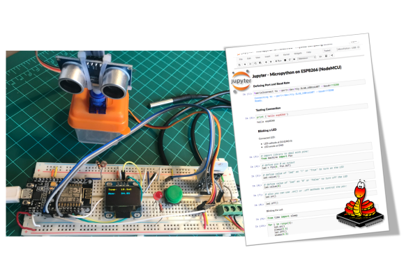
Let’s play with MicroPython on an ESP using a Jupyter Notebook. Getting data from sensors and taking action in a physical world.

1. Introduction

On a previous article, we explored how to control a Raspberry Pi using Jupyter Notebook: Physical ComputIng Using Jupyter Notebook

It was a great experience, and once the project worked very well I thought, “how about to also test Jupyter Notebook on an ESP8266 (or even on ESP32) using MicroPython?”.

As we all know, the Jupyter Notebook is an open-source web application that allows you to create and share documents that contain live code, equations, visualizations and narrative text. Uses include data cleaning and transformation, numerical simulation, statistical modeling, data visualization, machine learning, and much more. For “much more”, we have also explored “Physical Computing”.

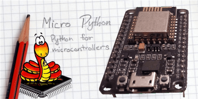
So far on my projects, I have mostly explored IoT and physical computing projects using ESP8266–01, 8266–12E (NodeMCU) and ESP32 programmed by an Arduino IDE, using its C/C++ type language. But another great tool to be used on programming those devices is MicroPython:

MicroPython is a lean and efficient implementation of the Python 3 programming language that includes a small subset of the Python standard library and is optimised to run on microcontrollers and in constrained environments. It aims to be as compatible with normal Python as possible to allow you to transfer code with ease from the desktop to a microcontroller or embedded system.

Also, I think that using Jupyter Notebook to program an ESP device using MicroPython, can be a great tool to teach Physical Computing to kids and also help scientists to quickly access real-world playing with sensors on acquiring data.

This is what we will try to accomplish in this tutorial:

• Output a digital signal to Turn On/Off a LED
• Read a digital input from a button
• Output a PWM signal to fade a LED
• Control a Servo Motor position using a PWM output
• Reading Analog signal (Luminosity using LDR )
• Reading Temperature vai 1-Wire (DS18B20)
• Reading Temperature and Humidity (DHT22)
• Displaying data using an OLED via I2C bus.

2. Installing MicroPython

The first thing to do with a fresh NodeMCU (or ESP32), is to erase wherever it is loaded in its memory and “flash” a new firmware, that will be the MicroPython interpreter.

A. Getting the new FW:

Go to the site: MicroPython downloads and download the appropriated FW for your device:

For example, for ESP8266, the latest version is:

esp8266-20180511-v1.9.4.bin (Latest 01Jun18)

(you can find details how to install the FW here)

The ideal is to create a directory where you will work with MicroPython. For example, in case of a mac, starting from your root directory:

cd Documents
mkdir MicroPython
cd MicroPython

B. Move the downloaded ESP8266 firmware to this recently created directory.

At this point:

Connect your NodeMCU or ESP32 on your PC using the serial USB cable.

C. Check where is the serial port that is being used by your device using the command:

ls /dev/tty.*

In my case, I got:

/dev/tty.SLAB_USBtoUART

D. Install esptool (tool used to flash/erase FW on devices)

pip install esptool

E. Erase the NodeMCU flash:

esptool.py --port /dev/tty.SLAB_USBtoUART erase_flash

F. Flash the new FW:

esptool.py --port /dev/tty.SLAB_USBtoUART --baud 460800 write_flash --flash_size=detect 0 esp8266-20180511-v1.9.4.bin

Once you have the Firmware installed, you can play with REPL* on Terminal using the command Screen Serial comm with ESP:

screen  /dev/tty.SLAB_USBtoUART 115200
>>> print (‘hello ESP8266’)
>>> hello ESP8266

If you are at REPL: [Ctrl+C] to break a pgm [Ctrl+A] [K] [Y] to quit and return to the terminal.

* REPL stands for “Read Evaluate Print Loop”, and is the name given to the interactive MicroPython prompt that you can access on the ESP8266. You can learn more about REPL here.

3. Installing Jupyter MicroPython Kernel

To interact with a MicroPython ESP8266 or ESP32 over its serial REPL, we will need to install a specific Jupyter Kernel.

This is necessary to be done only once.

From Jupyter Documentation website, we can list all “ Community-maintained kernels”. There, we will be sent to :

Jupyter MicroPython Kernel

Once we have Python 3 installed on our machine (in my case it is a Mac), clone the repository to a directory using the shell command (ie on a command line):

git clone https://github.com/goatchurchprime/jupyter_micropython_kernel.git

Next, install the library (in editable mode) into Python3 using the shell command:

pip install -e jupyter_micropython_kernel

This creates a small file pointing to this directory in the python/../site-packages directory and makes it possible to “git update” the library later as it gets improved.

Things can go wrong here, and you might need “pip3” or “sudo pip” if you have numerous different versions of python installed.

Install the kernel into Jupyter itself using the shell command:

python -m jupyter_micropython_kernel.install

This creates the small file “.local/share/jupyter/kernels/micropython/kernel.json” that jupyter uses to reference it’s kernels.

To find out where your kernelspecs are stored, you can type:

jupyter kernelspec list

The Terminal PrintScreen show you the list of kernels that I have installed on my machine. Note that in my case I installed the MicroPython kernel using PIP3 command and so, the Kernel is not in the same directory that the other ones (I got an error when trying to install my kernel using PIP).

Now run Jupyter notebooks:

jupyter notebook

In the notebook click the New Notebook button in the upper right, you should see your MicroPython kernel display name listed.

On the first cell, you will need to define the port and baud rate that will be used (115200 works fine):

%serialconnect to --port=/dev/tty.SLAB_USBtoUART --baud=115200

As a response, the cell will return:

Connecting to --port=/dev/tty.SLAB_USBtoUART --baud=115200
Ready.

And that’s it! When “Ready” appears, you should be able to execute MicroPython commands by running the cells.

Let’s try:

print ('hello esp8266')

You should receive the response of your ESP8266 as on output on the cell:

hello esp8266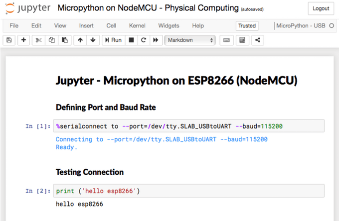

4. Blinking a LED

As usual, let’s start our journey to Physical computing, “blinking a LED”.

The available pins are: 0, 1, 2, 3, 4, 5, 12, 13, 14, 15, 16, which correspond to the actual GPIO pin numbers of ESP8266 chip. Note that many end-user boards use their own adhoc pin numbering (marked e.g. D0, D1, …).

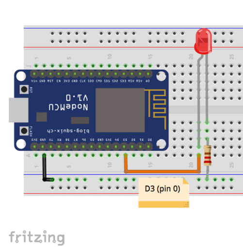
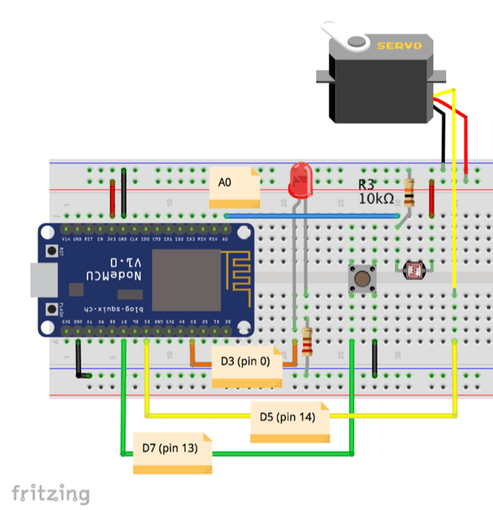
Install a LED on NodeMCU pin 0 (D3) and test it, turning it ON and OFF:

# import library to deal with pins:
from machine import Pin

# define pin 0 as output
led = Pin(0, Pin.OUT)

# define value of "led" as "1" or "True" to turn on the LED
led.value(1)

# define value of "led" as "0" or "False" to turn off the LED
led.value(0)

# also you can use .on() or .off methods to control the pin:
led.on()
led.off()

Now, Let’s import a time library and blink the LED:

from time import sleep

for i in range(5):
    led.on()
    sleep(0.5)
    led.off()
    sleep(0.5)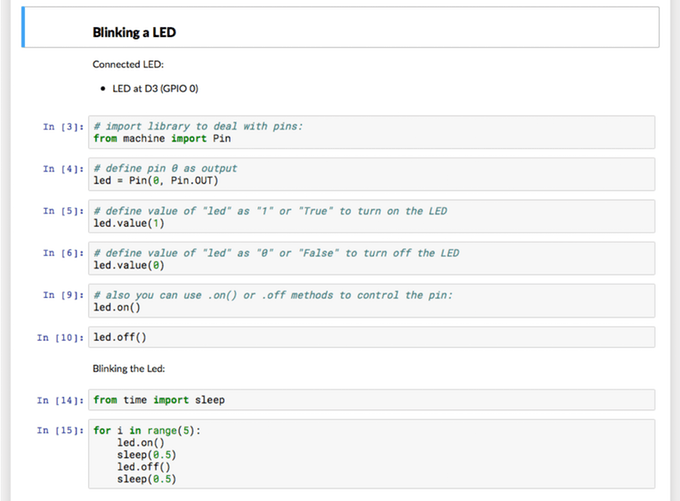

5. Input Digital Signal

The simple sensor data that you can read on a NodeMCU is a push-button.

Let’s install a push-button on a pin 13 (D7) as shown in the diagram.

Our push-button will be connected in a way that pin 13 normal state will be “High” (so we will use an internal Pull-up resistor to guarantee this state). When pressed, pin 13 will be “Low”.

# define pin 13 as an input and activate an internal Pull-up resistor:

button = Pin(13, Pin.IN, Pin.PULL_UP)

# Read button state:
print(button.value())

When you run the above cell, the result will be:

1

Pressing the button, run the cell again:

# Read button state:
print(button.value())

The result is now:

0

Note that stop pressing the button does not return the “cell value” to “1”. To see “1”, you must run the cell again.

Let’s now do a small program to turn ON the LED only if the button is pressed:

print (button.value())
if button.value() == 0:
    led.on()
else:
    led.off()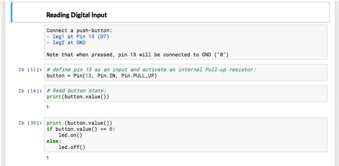

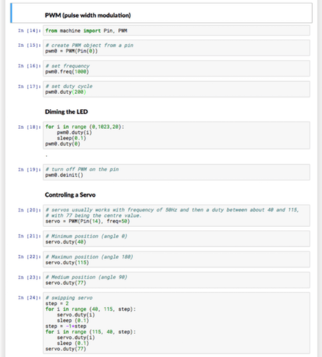
6. PWM (pulse Width Modulation)

PWM can be enabled on all pins except Pin(16). There is a single frequency for all channels, with a range between 1 and 1000 (measured in Hz). The duty cycle is between 0 and 1023 inclusive.

Start calling the appropriate library:

from machine import Pin, PWM

several commands are available:

pwm0 = PWM(Pin(0))      # create PWM object from a pin
pwm0.freq()             # get current frequency
pwm0.freq(1000)         # set frequency
pwm0.duty()             # get current duty cycle
pwm0.duty(200)          # set duty cycle
pwm0.deinit()           # turn off PWM on the pin

Or you can set configure the pin at once:

pwm2 = PWM(Pin(2), freq=500, duty=512)

Let’s dimming the LED connected to Pin 0 from OFF to ON:

from machine import Pin, PWM
pwm0 = PWM(Pin(0), freq=1000, duty=0)
for i in range (0,1023,20):
    pwm0.duty(i)
    sleep(0.1)
    pwm0.duty(0)
    pwm0.deinit()

And how about to control a Servo Motor?

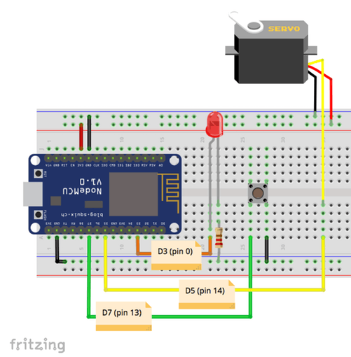
Let’s install a small hobby servo on our NodeMCU as shown in the diagram. Note that I am connecting the Servo VCC to NodeMCU +3.3V. This is OK for this tutorial, but on real projects, you must connect the Servo VCC to an external +5V Power supply (do not forget to connect the GNDs to NodeMCU GND).

The servo data pin will be connected to NodeMCU pin 14 (D5).

Servos usually work with frequency of 50Hz and then a duty cycle between about 40 and 115 will position them from 0 to 180 degrees respectively. A duty cycle of 77 will position the servo on its center value (90 degrees).

servo = PWM(Pin(14), freq=50)

Test the servo on different positions:

# Minimum position (angle 0)
servo.duty(40)

# Maximun position (angle 180)
servo.duty(40)

# center position (angle 90)
servo.duty(40)

You can also create a simple swapping program to test your servo:

# swipping servo
step = 2
for i in range (40, 115, step):
    servo.duty(i)
    sleep (0.1)
    step = -1*step

for i in range (115, 40, step):
    servo.duty(i)
    sleep (0.1)
    servo.duty(77)

Below the result:

I am not using the sonar here, so I will leave to you to develop a code to use it. It’s simple alheady! Try it!

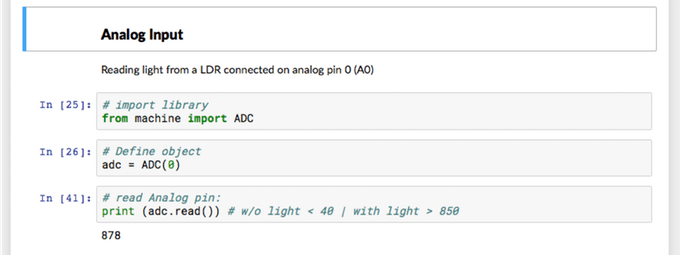
7. Analog Input (measuring Luminosity)

The ESP8266 has a single pin A0 which can be used to read analog voltages and convert them to a digital value. You can construct such an ADC pin object using:

from machine import ADC
adc = ADC(0)

Next, you can read the value of A0 pin using:

adc.read()

The Analog pin could be used to read, for example, a variable value got from a potentiometer as a voltage divider. This can be translated as an output for dimming the LED or move the servo to a specific position. You can try it based on what we have learned so far.

Another useful example is to capture data from an analog sensor, as temperature (LM35), ultraviolet (UV) radiation (as discussed in this tutorial) or luminosity using an LDR (“Light Dependent Resistor).

An LDR decreases its resistance when the luminosity increase. So, you can create a voltage divider with an LDR and a resistor as shown in the diagram.

Reading the analog voltage directly over the resistor, we will get a signal directly proportional to luminosity. leave the sensor exposed to light and read the ADC value. Cover the sensor and get a lower value.

In my case:

• Maximum Light ==> adc value > 850
• Minimun Light ==> adc value < 40

8. Controlling 1-Wire Devices

The 1-wire bus is a serial bus that uses just a single wire for communication (in addition to wires for ground and power). The DS18B20 temperature sensor is a very popular 1-wire device, and here we show how to use the onewire module to read from such a device.

For the following code to work you need to have at least one DS18B20 temperature sensor with its data line connected to GPIO 2 (D4).

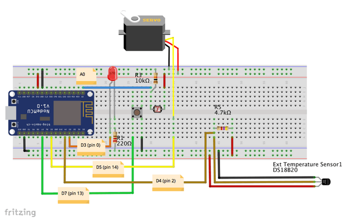
You must also power the sensors and connect a 4.7k Ohm resistor between the data pin and the power pin as shown in the diagram.

Import the libraries:

import onewire, ds18x20

Define which pin the 1-wire device will be connected. In our case ==> pin 2 (D4)

dat = Pin(2)

Create the onewire object:

ds = ds18x20.DS18X20(onewire.OneWire(dat))

Scan for devices on the bus. Remember that you can have multiple devices connected at same bus.

sensors = ds.scan()
print('found devices:', sensors)

“sensors” is an array with the address of all 1-wire sensors connected. We will use “arrays[0]” to point to our sensor.

Note that you must execute the convert_temp() function to initiate a temperature reading, then wait at least 750ms before reading the value (do not forget to import time library). To read the value use: ds.read_temp(sensors[0]):

ds.convert_temp()
time.sleep_ms(750)
print(ds.read_temp(sensors[0]))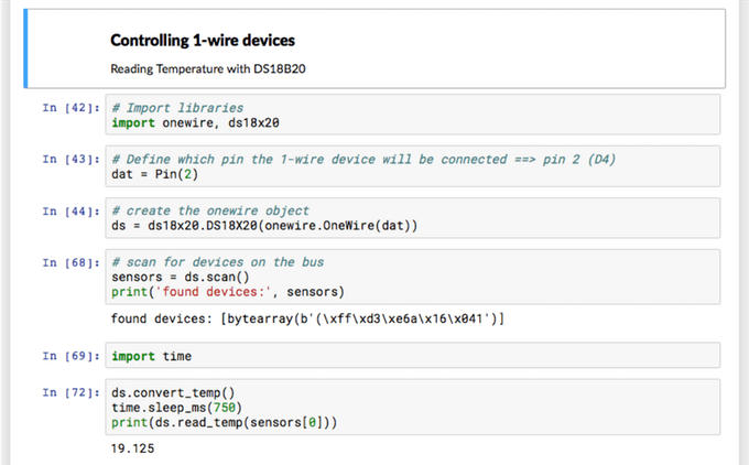

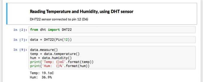
9. Reading Temperature and Humidity, Using DHT Sensor

DHT (Digital Humidity & Temperature) sensors are low-cost digital sensors with capacitive humidity sensors and thermistors to measure the surrounding air. They feature a chip that handles analog to digital conversion and provides a digital interface using only a single data wire. Newer sensors additionally provide an I2C interface.

The DHT11 (blue) and DHT22 (white) sensors provide the same digital interface, however, the DHT22 requires a separate object as it has a more complex calculation. DHT22 have 1 decimal place resolution for both humidity and temperature readings. DHT11 have whole number for both. A custom protocol is used to get the measurements from the sensor. The payload consists of a humidity value, a temperature value, and a checksum.

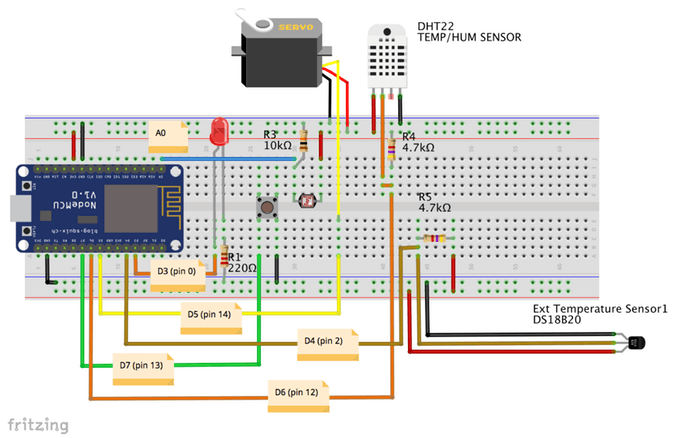
Connect the DHT22 as shown in the diagram. The data pin will be connected to NodeMCU pin 12 (D6).

To use the DHT interface, construct the objects referring to their data pin. Start calling the library:

from dht import DHT22

Define the appropriated pin and construct the object:

data = DHT22(Pin(12))

Get the Temperature and Humidity values:

data.measure()
temp = data.temperature()
hum = data.humidity()

print('Temp: {}oC'.format(temp))
print('Hum:  {}%'.format(hum))

The DHT11 can be called no more than once per second and the DHT22 once every two seconds for most accurate results. Sensor accuracy will degrade over time. Each sensor supports a different operating range. Refer to the product datasheets for specifics.

DHT22 sensors are now sold under the name AM2302 and are otherwise identical. 

10. I2C — Using an OLED Display

I2C is a two-wire protocol for communicating between devices. At the physical level it consists of 2 wires:

• SCL and SDA, the clock and data lines respectively.

I2C objects are created attached to a specific bus. They can be initialized when created or initialized later on.

First, let’s import the library:

from machine import I2C

Considering a device on Pin 4 (SDA) and Pin 5 (SCL), let’s create an i2c object:

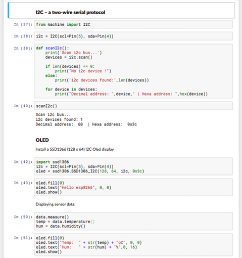
i2c = I2C(scl=Pin(5), sda=Pin(4))

Now, you should scan the I2C bus for eventual devices there. The function below will do this, returning the number of connected devices and its address:

def scanI2c():
    print('Scan i2c bus...')
    devices = i2c.scan()

    if len(devices) == 0:
        print("No i2c device !")
    else:
        print('i2c devices found:',len(devices))

    for device in devices:
        print("Decimal address: ",device," | Hexa address: ",hex(device))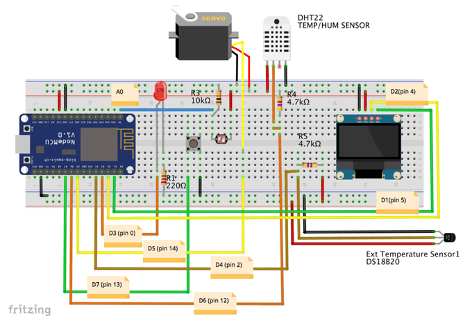

Let’s install an I2C OLED display on our NodeMCU as shown in the diagram. The display is the SSD 1306 (128 x 64).

Running the scan function:

scanI2c()

We will get as a result that 1device was found at address 0x3c.

This address will be used for an oled object creation as below:

import ssd1306
i2c = I2C(scl=Pin(5), sda=Pin(4))
oled = ssd1306.SSD1306_I2C(128, 64, i2c, 0x3c)

Some methods to manage the display:

poweroff(), turns off the screen. Convenient for battery operation.

contrast(), to adjust the contrast

invert(), invert the colors of the screen (finally white and black!)

show(), to refresh the view

fill(), to fill the screen in black (1) or white (0)

pixel(), to turn on a particular pixel

scroll(), scroll the screen.

text(), to display on text at the indicated x, y position

Draw lines hline(), vline() or any line line()

Draw a rect rect rectangle() or rectangle filled fill_rect()

Let’s test our display:

oled.fill(0)
oled.text("Hello esp8266", 0, 0)
oled.show()

And now, let’s display the DHT22 sensor data on put OLED:

data.measure()
temp = data.temperature()
hum = data.humidity()

oled.fill(0)
oled.text("Temp:  " + str(temp) + "oC", 0, 0)
oled.text("Hum:   " + str(hum) + "%",0, 16)
oled.show()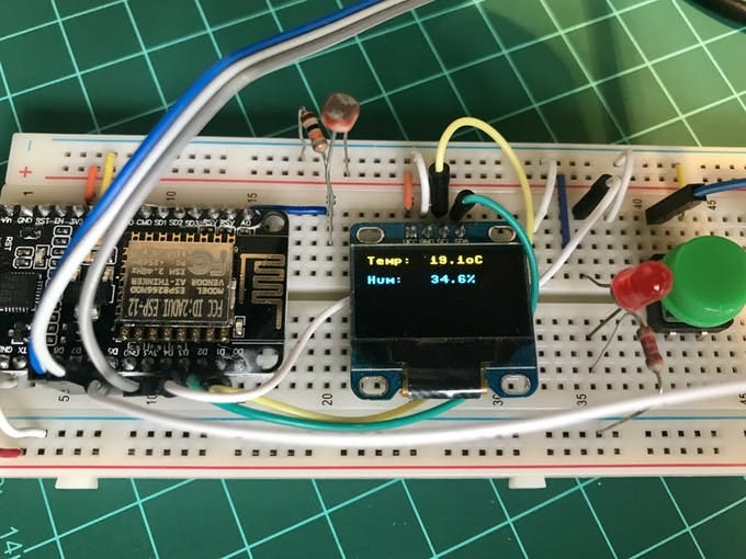

11. Going Further

This article deliveres the bits and pieces for you to build a more robust project, using MicroPython as a programming language and Jupyter Notebook as a tool for quick development and analysis.

Of course, if you want to run a program written in MicroPython on a NodeMCU independent of your PC and Jupyter, you must save your code as a “main.py” file for example, in any text editor and download it on your device using: “ Ampy”, that is a utility developed by Adafruit, to interact with a MicroPython board over a serial connection.

Ampy is meant to be a simple command line tool to manipulate files and run code on a MicroPython board over its serial connection. With ampy you can send files from your computer to a MicroPython board’s file system, download files from a board to your computer, and even send a Python script to a board to be executed.

Installation:

sudo pip3 install adafruit-ampy

Ampy is made to talk to a MicroPython board over its serial connection. You will need your board connected and any drivers to access it serial port installed. Then, for example, to list the files on the board run a command like:

ampy --port /dev/tty.SLAB_USBtoUART ls

For convenience, you can set an AMPY_PORT environment variable which will be used if the port parameter is not specified. For example on Linux or OSX:

export AMPY_PORT=/dev/tty.SLAB_USBtoUART

So, from now one, you can simplify commands:

List internal NodeMCU files:

ampy ls

You can read a file installed on your nodeMCU using:

ampy get boot.py

Once you create a file using your text editor (nano for example), you can install it on your NodeMCU using:

ampy put main.py

Now, when you press “Reset” button on your NodeMcu, the program that will run first is “main.py”.

For Windows, please see the Adafruit instructions here.

12. Conclusion

As always, I hope this project can help others find their way into the exciting world of electronics!

For details and final code, please visit my GitHub depository: Pyhon4DS/Micropython

Saludos from the south of the world!

See you in my next article!

Thank you,

Marcelo